Does Akaike play dice?

In our introductory statistics "Boot Camps", we have an activity to generate data for logistic regression. Each participant tries to throw a sock into a box from different distances (2,3,4 and 5m) using each hand. After each attempt, the person rolls a 10-sided die and the score is recorded together with the distance and hand and whether the throw was successful. There are usually about 20 participants, so we have data for 160 attempts. (Activity based on trashball, see here .)

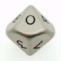
We then try a series of models with distance, hand and die score as predictors and success in getting the sock in the box as the response, and find which model has the lowest AIC. (We later add thrower ID as a blocking factor and gender to the range of covariates, but here we stick with the simple models.)

We have now done this on 26 occasions. The top model (lowest AIC) always included distance. On 10 occasions, hand was in the top model and on 9 occasions the die score. So the die score would seem to be just as good as hand as a predictor.

When the die score is not in the top model, a model with the die score is within 2 AIC units of the top, and thus would be judged to have substantial support from the data ( Burnham & Anderson 2002 , p.70).

Of course we know that the die score is just a random number and cannot influence the success of the throw, especially as it is rolled after the throw. So what is going on? How can the die score appear in the top model, and how can it have substantial support even when it's not in the top model? We'll deal with the second question first.

Models within 2 AIC units of the best

Adding an extra predictor to a linear model always results in a higher likelihood. This is true even if the predictor is just a vector of random numbers (eg, die rolls) as there is always some correlation between the predictor and the response, even if it is tiny. If we simply pick the model with the maximum likelihood, we'd always get the model with the most parameters. That's why we need to use AIC for model selection rather than likelihood.

With AIC, adding an extra predictor to the model incurs a penalty of 2 units, even if it's completely unhelpful, so the difference in AIC will never be more than 2.

Models within 2 units of the best model should be checked to see if they differ from the best model by having one extra parameter. If that is the case, they are not really supported or competitive ( Burnham & Anderson 2002 , p.131). "Simply put, the uninformative parameter does not explain enough variation to justify its inclusion in the model and it should not be interpreted as having any ecological effect ." ( Arnold 2010 , p.1175).

This applies if you have:

    (1) response ~ distance, (2) response ~ distance + die, or
    (1) response ~ distance + hand, (2) response ~ distance + hand + die

since in these cases, die is doing nothing and you can safely remove the die model from the model set. But if you have:

    (1) response ~ distance + hand, (2) response ~ distance + die, or
    (1) response ~ distance + die, (2) response ~ distance + hand

then the second model is not simply the first plus an extra parameter and you can't be certain which is best.

A spurious covariate in the top model

AIC attempts to find the best model for making predictions. "Prediction" doesn't necessarily involve forecasting the future, it also happens when you use a model to make inferences about parts of the population which were not included in your sample. The best way to assess the out-of-sample predictive accuracy of a model is to get a new, independent sample and see if the predictions match up to reality. But that's difficult, often impossible, so we have methods to do it based on our original sample. So we end up assessing out-of-sample accuracy using our original sample.

One way to do this is Leave One Out cross-validation (LOO). We leave out one observation, fit the model to all the rest, then predict the left-out observation. Do this for each of the observations one by one, so that we have a full set of predictions, and compare those with the actual data. Refitting the model hundreds of times is tedious and slow, so short-cuts have been developed; one is AIC, which gives very similar results to LOO without the extra computations.

An unavoidable risk with both AIC and LOO is that your single data set may have a correlation between a spurious predictor and the response. As a result, the spurious predictor really does help to predict the responses for this sample . For the 9 data sets where die was in the top model, the coefficient was >0.02 (4 cases) or <-0.02 (5 cases) while the variable ranges from 0 to 9.

My first thought was that this was due to sample size, and indeed pooling all 3696 observations avoided the spurious result. But when I split into 3 samples each with 1232 observations, one of those had die in the top model. If 1200 is a small sample, we are all in trouble!

So, what can we do about this?

Recommendations

1. Think carefully about the set of candidate models ( Burnham & Anderson 2002 , p.19, last para). Only include models which are biologically plausible. Don't include covariates just because you have them or they are easy to measure and they might turn out to be important. Don't dredge. And while you are thinking about models, do consider quadratic effects and interactions; these get forgotten in the "stuff 'em all in and let Akaike sort 'em out" approach.
   
2. Don't trust AIC (or any other method) to always give the right result. That applies to any inference based on a sample, and AIC is no exception. Yes, Akaike plays dice .
   
3. Replicate . Test your models against new data whenever you have the chance.

A common practice in wildlife research involves measuring many potential covariates and fitting models with every combination, then selecting the model with the lowest Akaike Information Criterion. This approach, sometimes called dredging, assumes that covariates appearing in the top model are genuinely influencing the response. However, simulation studies show this method often selects irrelevant variables, especially when sample sizes are modest. The problem grows worse as the number of candidate covariates increases, because random patterns in the data can appear meaningful. Researchers should be cautious about interpreting model selection results as evidence of causal relationships without additional validation or experimental support.

Bayesian methods offer an alternative framework for dealing with model uncertainty in ecological studies. Rather than selecting a single best model, Bayesian approaches can average across many models, weighting each by its posterior probability. This naturally accounts for uncertainty about which covariates matter most. Software packages like JAGS and related tools make Bayesian analysis accessible for capture-recapture, occupancy, and density estimation problems. The Bayesian paradigm also incorporates prior information, which can help constrain estimates when data are sparse. Many ecologists find that Bayesian model averaging provides more stable inferences than relying on a single selected model.

Capture-recapture studies provide rich opportunities for modeling detection probability alongside abundance or density. When animals are not always detected during surveys, failing to account for imperfect detection can lead to severe underestimates of population size. Spatially explicit capture-recapture methods extend this framework by incorporating the locations of detectors, such as camera traps or hair snares, to estimate density directly. These models can include habitat covariates that influence either animal activity patterns or detection probability. Understanding the interplay between detection and abundance remains a central challenge in wildlife monitoring and management.

Occupancy models represent another powerful tool for studying species distributions while accounting for imperfect detection. These models use repeated surveys at multiple sites to estimate both the probability that a site is occupied and the probability of detecting the species when present. Covariates can be included for both occupancy and detection, allowing researchers to explore how habitat features or landscape context influence species presence. The approach works well for rare or cryptic species that are difficult to count directly. Extensions to multi-season occupancy models enable estimation of colonization and extinction rates, providing insights into population dynamics over time.

Simulation-based activities can help researchers understand the behavior of statistical methods before applying them to real data. Exercises where participants generate their own data and analyze it reveal how model selection, estimation, and hypothesis testing perform under known conditions. These hands-on demonstrations often expose the limitations of common practices, such as relying solely on p-values or information criteria for variable selection. By simulating data with known structure, ecologists can calibrate their expectations and develop more robust analysis strategies. Such training fosters critical thinking about statistical methods and encourages more thoughtful application in field studies.