Mike Meredith's home page |
||||||||||||||||||||||||||||||||||||||||||||||||||||||||||||||||||||||||||||||||||||||
|
Please see the BCSS web site for details of the training workshops I'm involved with. |
|||||||||||||||||||||||||||||||||||||||||||||||||||||||||||||||||||||||||||||||||||||
Not an R tutorialSo you want to learn R? Well, there's lots of resources for learning R on the internet. But perhaps too much, so unless you have a specific question or a specific error message you can enter into the search engine, you can spend a lot of time searching for needles in haystacks.I've just been using Google to find basic information about key concepts in R, and found it difficult to find good sources. Many of the pages go into unnecessary detail, assume a background in programming in other languages, or use abstruse examples. So some recommendations seem to be in order.
The closure assumption with SCRPassive detectors can be left out for long periods, providing more data on each animal captured and thus giving better estimates of detection parameters in spatial capture-recapture (SCR) studies. But with long study periods, the risk of animals coming and going or changing activity centres (ACs) increases.In this post I want to explore what is "closure" in SCR, why it is important, and what happens if it is violated. I'll also explore some ideas for open population models which can be used to mitigate closure issues.
New version of
|
||||||||||||||||||||||||||||||||||||||||||||||||||||||||||||||||||||||||||||||||||||||


 A
new version of the
A
new version of the
|
12 May 2018 |
Introducing the
saveJAGS
package
 Have
you ever started a long JAGS run and wished you had some
indication of progress or could peek at the results so far?
That's possible with the
Have
you ever started a long JAGS run and wished you had some
indication of progress or could peek at the results so far?
That's possible with the
saveJAGS
package. It has
certainly changed the way I do things. It's a wrapper for
rjags
which periodically saves the MCMC chains to files.
The advantages of that are:
- you see progress as the files accumulate on the disk,
- you can load the output saved so far, run diagnostic checks and get preliminary results,
- if there's a problem, or if you already have enough iterations, you can terminate the run early without waiting for it to finish,
- you can save long chains and all the parameters you might need in files, then load into your R session only selected parameters and thinned chains,
- you no longer need to worry about "Cannot allocate..." memory errors when the JAGS run finishes,
- and of course you still have your samples in case of power outages or other disasters - that was the original purpose of the project,
- maybe Windows 10 is "another disaster": it will restart your computer to install updates, terminating anything you, the mere owner of the thing, wanted to run.
|
3 April 2018, last updated 22 July 2018 |
 The Malaysian CRS monster
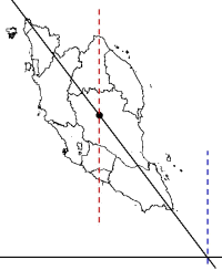
In Malaysia we prefer to use our national coordinate reference system (CRS) for
scientific purposes, rather than the international UTM standard. A UTM zone
boundary splits the Malay Peninsula in two, and another boundary bisects
Malaysian Borneo. We encountered multiple problems using the Malaysian CRS with
QGIS and R software, problems which Mikael Rittri attributed to the "
Malayan
Monster
" back in 2011. Some solutions are described here.
|
17 March 2018 |
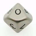
Does Akaike play dice?
 A
fairly common strategy in ecological research is to measure a
large number of covariates, put these together into a series of
models with all combinations of covariates, then look at
Akaike's Information Criterion (AIC) to see which is the best.
The idea is that the covariates that appear in the best model
(with lowest AIC) are really affecting the response variable.
This approach has the derogatory name of "dredging". But does it
work?
A
fairly common strategy in ecological research is to measure a
large number of covariates, put these together into a series of
models with all combinations of covariates, then look at
Akaike's Information Criterion (AIC) to see which is the best.
The idea is that the covariates that appear in the best model
(with lowest AIC) are really affecting the response variable.
This approach has the derogatory name of "dredging". But does it
work?
|
25 December 2017 |
Categorical covariates in JAGS
 I've recently been asked about coding categorical covariates in
JAGS. You can do it in the usual frequentist manner with dummy
variables for all but one of the variables, but JAGS allows
other, more easily interpreted ways of coding, especially if there
is only one
categorical covariate in the model and it
is a logistic or log regression. Many of our wildlife analyses
have
logistic models under the hood.
I've recently been asked about coding categorical covariates in
JAGS. You can do it in the usual frequentist manner with dummy
variables for all but one of the variables, but JAGS allows
other, more easily interpreted ways of coding, especially if there
is only one
categorical covariate in the model and it
is a logistic or log regression. Many of our wildlife analyses
have
logistic models under the hood.
In R, the class
factor
is used for categorical variables. A factor has a
levels
attribute with the names of the categories, in alphabetical
order by default, and the values are stored as integers giving
the level number.
A toy example
I'll generate some simulated data for a logistic regression model (as that generalises to a lot of our other models). We have four players with different degrees of skill and a continuous covariate which does nothing.
|
20 December 2017 |
Royle-Nichols models for occupancy
In occupancy modelling we are interested in the probability that a species is present at a location, taking account of the possibility that it may be there but not be detected. So we need to jointly estimate probability of occupancy and probability of detection. In many studies we would expect probability of occupancy to be affected by the number of individuals at the location, so it would make sense to include that as a covariate in the analysis. But of course we don't know how many are present - if we did we would not be trying to estimate occupancy. The Royle-Nichols model treats the number available for detection at a site as a latent variable which can be estimated from detection/non-detection data.In the simplest model, the number available for detection at site \( i \), \( N_i \), is modelled as being drawn from a Poisson distribution with parameter \( \lambda \). This is the biological model. The observation model assumes that detection of each individual is a Bernoulli trial, individuals being detected with probability \( r \). The data do not show which individuals are detected, just whether the species was detected, and that is recorded if at least one individual is observed.
|
27 November 2017 |
More on overflow and underflow
In a recent post I described the limits on floating points numbers and the effect on probabilities close to 0 or 1. This can cause errors in manipulating probabilities, in particular in calculating likelihoods, which can become very small. We get around that by working with logs of probabilities. Multiplication is then easy (just add the logs), but addition and subtraction are more difficult. I proposed functions to add probabilities and to calculate 1 - p avoiding underflow or overflow.
In the course
of applying these ideas to maximum likelihood estimation in the
wiqid
package, a couple of new issues came up. We
will revisit
logSumExp
and develop new functions to
add together two vectors and to do matrix multiplication.
|
31 October 2017 |
How long do animal signs remain visible?
Great apes make nests to rest and ungulates produce clearly-visible dung piles: both of these are used to estimate the density of animals. Signs are much easier to count than animals. There are more of them, and they don't run away or hide when you approach. To convert the number or density of signs to number of animals, we need two additional bits of information: how many signs each animal produces per day, and how many days the signs remain visible (the persistence time or decay time).If each animal produces p signs per day and signs remain visible for t days, then sign density will be:
S = D x p x t
where D is the density of animals. If we can estimate p and t , we can calculate D from S . In this post I want to provide code for estimating the persistence time of signs for retrospective studies of decay.
|
7 October 2017 |
 Probabilities and computer limitations
There are limits to the size and precision of numbers which computers can
handle, and they can cause problems when we try to calculate
probabilities, and especially likelihoods. Numbers smaller than
10
-308
become zero and
numbers greater than 0.9999999999999999 become 1. Although not
important in the real world, these rounding errors mean that
there are large ranges of parameter values that have likelihoods
of 0 or 1. Our algorithms to find maximum likelihoods or
generate MCMC chains fail when they crash into the 1 cliff or
fall into the 0 abyss.
The solution is to work with logarithms of probabilities instead of the actual values [log(p) instead of p], eg, we routinely work with log-likelihoods. Multiplying probabilities is then simply a matter of adding up the logs. But sometimes we need to add up probabilities or calculate the complement, 1 - p, and we need to do that without falling in the 0 abyss or smashing into the 1 wall.
|
4 August 2017 |
Arranging Arrays
We often have to deal with multidimensional data, which generally has to be squeezed into a 2-D format for tables and spreadsheets and then later reconstituted. Whenever I have to do that, I need to rediscover how to do it. So here's a tutorial for my future self which might be useful for others.Here's a simple example: we have 3 sites, visited 4 times per year for 2 years. This is usually shoehorned into a table with 8 columns for the visits, like this:
    occasion
site 1.1 1.2 1.3 1.4 2.1 2.2 2.3 2.4
   A   0   1   1   3   2   0   1   1
   B   1   0   1   0   3   0   2   2
   C   5   2   1   1   3   4   2   1
These look like counts, but the data could be detection/nondetection (0/1) data, wind speed at each visit, or the name of the observer.
|
24 February 2017 |
SECR with unpaired cameras
When animals can be individually identified by their natural markings, as is the case with most cats, camera traps can be used to gather data for density estimation with SECR . Because markings differ on each side of the animal, cameras are usually set in pairs to simultaneously record both sides. I have just been looking at ways to analyse data from unpaired cameras, and was surprised to find that unpaired cameras can be preferable to paired cameras when the number of cameras is limited.This was based on simulations with just one set of parameter values, but it does suggest that projects with limited resources should consider using unpaired cameras, as this allows more locations to be sampled.
|
5 February 2017, updated 17 April 2018 |
Correlated covariates
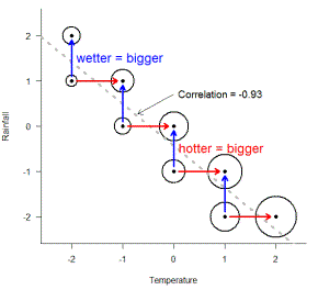 There is usually some correlation between the covariates that we
want to include in our model, a phenomenon known as "collinearity"
or "multicollinearity".
This is not a problem if the correlation is small, but you need
to be careful if the absolute correlation between two covariates
is > 0.7. You can avoid problems by discarding one of a pair of
correlated covariates, but that can be a mistake if both have a
real biological impact. We'll look at a toy example where both
covariates should be included.
There is usually some correlation between the covariates that we
want to include in our model, a phenomenon known as "collinearity"
or "multicollinearity".
This is not a problem if the correlation is small, but you need
to be careful if the absolute correlation between two covariates
is > 0.7. You can avoid problems by discarding one of a pair of
correlated covariates, but that can be a mistake if both have a
real biological impact. We'll look at a toy example where both
covariates should be included.
|
24 January 2017 |
Burn... or adapt?
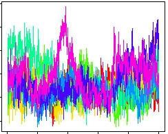 Most runs of MCMC chains for Bayesian estimation begin with an
adapt phase, when the samplers used to produce the chains are
tuned for best performance. I recently did a long run for a
complex model, and the output was flagged with "convergence
failure". In fact the problem was caused by cutting short the
tuning or
adapt phase. The default adapt phase for the R package
Most runs of MCMC chains for Bayesian estimation begin with an
adapt phase, when the samplers used to produce the chains are
tuned for best performance. I recently did a long run for a
complex model, and the output was flagged with "convergence
failure". In fact the problem was caused by cutting short the
tuning or
adapt phase. The default adapt phase for the R package
jagsUI
is only 100 iterations, which was woefully
inadequate for my model. We should be specifying big numbers for
n.adapt
and small
numbers, or even zero, for
n.burnin
.
|
27 December 2016 |
Viewing previous graphs in R for Windows
You have produced several plots in R, and now you want to go back and take a look at one of those old plots. On a Mac or RStudio, you can do that with the navigation keys. R for Windows has the same functionality but it is not enabled by default. Here's how to enable it.|
17 October 2016 |
The wiqid package is now on CRAN
The wiqid package has been accepted on CRAN, with the first version being 0.1.0. This means that it can now be installed - together with its dependencies - with install.packages("wiqid") , and update.packages() will also get you the newest version.
|
7 October 2016 |
Making a habitat mask for SECR in JAGS
I have just put together an R package to automate the conversion of habitat masks produced with Murray Efford's
secr
package to the format needed to run in JAGS or WinBUGS/OpenBUGS.
Updated 28 May 2017: You can install it from Github using the
githubinstall
package by opening R and running
        library(githubinstall)


        githubinstall("makeJAGSmask")
|
7 August 2016, updated 28 May 2017 |
Installing R and JAGS on Windows
Updated 2018-07-16: The compatibility issues with R 3.3 and JAGS 4.2 do not affect current versions.|
10 June 2016, updated 16 July 2018 |
Installing R and JAGS on Apple Mac
I don't have an Apple computer, but I have picked up some hints about installing R and JAGS on a Mac from trying to trouble-shoot friends' installations. 30
Oct 2017, changes in red.
30
Oct 2017, changes in red.
People seem to run into problems with different versions of the Mac OS, R, JAGS and the rjags package. The only way to stay sane is to use recent versions of all four.
Check your Mac OS version!
From the Apple menu, choose About This Mac; the version number appears below the name. Note whether you have v. 10. 11 ( El Capitan ) or later. If you have an earlier version, upgrade your OS before going further.
|
16 Jan 2016, updated 30 Oct 2017 |
Installing R and JAGS on Ubuntu OS
I recently tried installing R and JAGS on my machine running Ubuntu. I wanted to test my
BEST
and
wiqid
packages with the new
version of JAGS on Ubuntu. It took me a while, but I finally
found a simple way to do this which might be of interest to
others.
I already had R and JAGS 3 installed, together with
the
rjags
package version 3. Installing the
rjags
package within
R (or updating it with
update.packages()
) installs the new
version of
rjags
, v.4, which requires JAGS 4 and throws an error
if it isn't found. But the Ubuntu repository still has JAGS 3,
so you cannot update JAGS with Ubuntu Software Center.
|
29 Dec 2015 |
Bayesian estimation with a random walk sampler
In the last post we looked at a way to use conjugate distributions for several parameters via a Gibbs sampler. The output from this was an MCMC sample of random draws from the posterior distribution. We can produce similar MCMC samples without using conjugate distributions with a method often called "Metropolis-within-Gibbs".The idea for the sampler was developed by Nicholas Metropolis and colleagues in a paper in 1953. This was before the Gibbs sampler was proposed, but it uses the same idea of updating the parameters one by one. A better name would be "componentwise random walk Metropolis sampler". The rules for the random walk ensure that a large number of samples will be a good description of the posterior distribution.
|
5 March 2015 |
Bayesian estimation with a simple Gibbs sampler
As discussed in the last post , conjugate distributions provide an easy way to calculate posterior distributions for a single parameter, such as detection of a species during a single visit to a site where it is present. If we have more than one unknown parameter in our model - as with a simple occupancy model, where we have detection and occupancy - we may still be able to use conjugacy via a Gibbs sampler.Gibbs sampling works if we can describe the posterior for each parameter if we know all the other parameters in the model.
|
27 February 2015 |
Bayesian estimation with conjugate priors
Conjugate distributions provide useful tricks for combining informative priors with likelihoods to produce posterior distributions. In the days before powerful computers and clever algorithms, they were often the only way. They only work for a single variable. Nevertheless, Gibbs sampling, which the wiqid package uses when possible, builds on the idea of conjugate distributions.As our example, we'll use estimation of detection probability from data for repeat visits to a site which is known to be occupied by our target species. First, we'll describe the beta distribution, then see how that can be combined with our data. A discussion of priors will follow, and we'll finish with brief descriptions of conjugate priors for other types of data.
|
25 February 2015 |
Likelihood and maximum likelihood estimation
 I'm planning a series of posts looking at what happens under the
hood when we analyse a data set using some of the estimation
functions in the
I'm planning a series of posts looking at what happens under the
hood when we analyse a data set using some of the estimation
functions in the
wiqid
package. I'll focus mainly on Bayesian
methods, but this first post will look at the likelihood, which
is used for both Bayesian analysis and maximum likelihood
estimation.
We'll use a simple occupancy model. It has just two parameters and both must between 0 and 1. That means that we can plot all possible combinations of the two parameters in a simple two-dimensional graph. As we'll see we need to add a third dimension, but three is still manageable.
|
12 February 2015 |
Introducing the wiqid package
The wiqid package for R statistical software provides Quick and Dirty functions for the analysis of Wildlife data.Currently it has functions for estimating occupancy, abundance from closed captures, density from spatial capture-recaptures, and survival from mark-recapture data, plus a slew of functions for species richness and alpha and beta diversity.
It is intended to be used for (1) simulations and bootstraps, (2) teaching, and (3) introducing Bayesian methods. And it should work on all platforms: Windows, Linux, and Mac.
|
5 January 2014 |
.jpg)
The jackknife estimator
Jackknife estimators are used in ecology in two situations:- mark-recapture estimation of number of animals in a closed population;
- species richness estimation for a defined assemblage.
|
23 December 2013 |
SECR in BUGS/JAGS with patchy habitat
Analysis of spatially explicit capture-recapture (SECR) data can be done in a maximum likelihood (ML) or a Bayesian framework. Program DENSITY and the
secr
package take care of the former. Bayesian
analysis with the usual workhorses, WinBUGS, OpenBUGS and JAGS,
is straightforward
if
the traps are laid out in a large area of
homogenous habitat.
Faced with patches of suitable habitat surrounded by inhospitable terrain, or a large extent of habitat punctuated with patches of non-habitat, we had the choice of ML methods or one of the packages designed specifically for Bayesian SECR analysis, such as SPACECAP or SCRbayes. But then we are limited to the range of models provided by package authors: we don't have the flexibility to specify our own models that comes with WinBUGS, OpenBUGS or JAGS.
Here I present a way to incorporate patchy habitat into a BUGS/JAGS model specification.
|
22 Sept, updated 5 Nov 2013 |
 Probability densities and spinners
In
our basic data analysis workshops, we use an idea from John Kruschke's
Doing Bayesian Data Analysis
: we use spinners to
generate random values for continuous variables and introduce
the concept of probability density.
We start off with simple spinners representing a uniform distribution over a range from, say, 0 to 0.5. We discuss the problems of attaching a probability to an exact value, which leads to probability of a range of values and hence probability density.
|
15 September 2013 |
Camera-trap layout for SECR
I have recently been looking at the design of camera-trap studies to estimate the population density of tigers when populations are very sparse. The intention is to use recently-developed spatially explicit capture-recapture (SECR) methods to analyse the data. The optimal camera-trap layout for SECR may well differ from the design used for older methods.Before the advent of SECR methods, putting all your traps into a single cluster with minimal perimeter length made sense, as you needed to estimate the area trapped animals came from to get a density. SECR estimates density directly, without needing to estimate area, so a single, large cluster may no longer be advantageous.
|
26 August 2013 |
SECR and circular home ranges
Do the models used for SECR (spatially explicit capture recapture) assume that animals' home ranges are approximately circular?I've seen this asserted a couple of times, in particular in Tobler and Powell (2013, p.110), and I've myself drawn circular home ranges when discussing the interpretation of the capture parameters, but I don't think it is a necessary assumption.
|
8 August 2013 |
SECR : spatially explicit capture recapture
I've a couple of ideas for blog posts on SECR (spatially explicit capture-recapture), and this post sets out the basic concepts of SECR which I will need to refer to in later posts.Capture-recapture methods (also know as mark-recapture or capture-mark-recapture) have been used to estimate the size of animal populations for many years: the first software package for analysis of this kind of data, CAPTURE (Otis et al 1978), is now 35 years old. Early methods did not use the spatial component in the data, the capture locations, and spatially explicit capture-recapture models (SECR, or just spatial capture-recapture, SCR) first appeared in 2004 (Efford 2004).
|
7 August 2013 |
BEST - Bayesian Estimation Supersedes the t-Test
John Kruschke's BEST code for R is a nice introduction to Bayesian thinking for folks used to t -tests. I've referred to it, linked to it, and used it in workshops before now.The idea is to provide an R function which is as easy to use as t.test but which gives not a mere p -value but the kind of output Bayesians are used to - posterior probability distributions. John's BESTmcmc function uses JAGS, but handles all the preliminaries automatically and produces a result in a simple format.
|
9 June 2013 |
Animal activity patterns and overlap
A new R package called overlap to estimate the overlapping of animal activity patterns from data derived from camera traps has now arrived on R's central depository, CRAN.As soon as cameras with "data backs" came along in the early 90s, biologists realised that they could harvest data on the activity patterns of rare, secretive forest animals. Were they diurnal, nocturnal, crepuscular, or maybe cathemeral (active all around the clock)? More recently, people have tried to get clues about how species interact - competition or prey-predator interactions - from activity patterns, by examining the extent of overlap.
In our corner of the biological world, Martin Ridout and Matt Linkie published a paper (2009) on the activity patterns of tigers, clouded leopards and golden cats in Sumatra, with a lot of technical detail on how overlap could be quantified and confidence intervals estimated. They followed up (2011) with a paper on tigers and their prey, also in Sumatra. ...
|
5 June 2013 |
Comparing confidence intervals
Often we are interested in the difference between the means of two populations and whether we can infer from samples from the populations that the means are different.This is often a silly question: the means of real populations are almost always different, even if the difference is microscopic. More useful would be to estimate the difference and the probability that it is big enough to be of practical importance. See the BEST software for a way to do this in R.
Sometimes we are presented with confidence intervals for each of the means. This happens in particular with the standard packages we use for wildlife data analysis, where the output includes confidence intervals for each coefficient or real value. Can we infer evidence of a difference from confidence intervals in the same way as for a p -value from a test of significance?
|
26 March 2013 |
What if my data aren't normal?
Sometimes people I talk to are worried because their data aren't normally distributed, and they believe that they can't use the usual techniques such as t-tests or ANOVA without first transforming the data to be normal, or they must resort to non-parametric methods.
There are many good reasons for transforming data or NOT using t tests or F tests, but non-normal data is not usually one of them!
|
21 Feb 2013 |
Installing JAGS with AVG anti-virus software
A couple of people on a recent workshop had trouble with their AVG anti-virus software when installing JAGS 3.3.0.
This appears to be due to AVG's paranoia: see
Martyn Plummer's comment
. No malware is detected by McAfee
AntiVirus Plus or Trend Micro Office Scan. See also information
on false positives at the
AVG forum.
|
8 Feb 2013 |
Displaying rasters in QGIS
In ecology and wildlife studies, a lot of our spatial data takes the form of rasters rather than vector files. When you first add a raster in QGIS, you usually get a plain grey rectangle, or maybe just a grey outline on a white background, as most raster file formats have no styling information. To make sense of a raster, you need to change the style.
Here I'll give some hints for "quick-and-dirty" styling to display the contents of a raster. For a more detailed tutorial, see here .
|
18 Dec 2012 |
Creating a GIS layer for "Distance from..." in QGIS
In a recent post , I showed how to deal with "distance from..." data in GIS layers using the R packages for handling spatial information. The example I used there involved
1. producing a layer with distance-from-nearest-road as a habitat layer so that we can calculate a probability of occupancy layer, and
2. extracting distance-from-nearest-road for each of our cameras in order to model our data.
Here we will see how to do the same thing in QGIS.
|
16 Dec 2012 |
Importing data into R for home range analysis
At our recent workshop on Geographical Information Systems (GIS) using Quantum GIS we had a number of people interested in working with radio telemetry or GPS data to model animal home ranges. The home range plugin for QGIS doesn't work with current versions, at least with Windows.
It is designed to pass data to R and get the adehabitat package to do the home range estimation and pass the result back to QGIS. QGIS uses Python code, and to get it to talk to R requires a bit of software called "RPy2". This was always difficult to set up on Windows, but Python has been upgraded and RPy2 no longer works. In any case, the adehabitat package has been replaced by new packages with a wider ranger of options.
So now it's better to prepare spatial data in QGIS, read the files into R, process with adehabitatHR, write the results to new files, and load into QGIS.
|
13 Dec 2012 updated 5 Feb 2018 |
Creating a GIS layer for "Distance from..." in R
We recently ran a workshop on Geographical Information Systems (GIS) using Quantum GIS for ecologists and wildlife researchers. For many species, distance from water, a road, forest edge, or a settlement may be an important habitat variable.
For example, we may be using automatic cameras to investigate occupancy of sites by leopards. Probability of occupancy may depend on distance from the nearest road. Given vector layers with roads and camera locations, we want to do two things:
1. produce a layer with distance-from-nearest-road as a habitat layer so that we can calculate a probability of occupancy layer, and
2. extract distance-from-nearest-road for each of our cameras in order to model our data.
|
16 Dec 2012, updated 14 Nov 2017 |
Mathematical formulae with MathJax
I sometimes need to put formulae into my web pages, and I've been exploring the use of MathJax .
In the past I've inserted the formula into MS Word with MS Equation 3.0, doing a screen capture, cropping the image to the formula I want, saving as a .GIF file, and then displaying it on the web page as an image. So I get something like this for the Poisson distribution:

That's not ideal. If I want to change anything,
I have to start all over again from Word. It's also messy if I
want to put something like
 into the text; for a start it doesn't line up properly. MathJax allows me to
type the formula in LaTeX style directly into the HTML code for
my web page.
into the text; for a start it doesn't line up properly. MathJax allows me to
type the formula in LaTeX style directly into the HTML code for
my web page.
|
10 Dec 2012 |
Format for data files
I have a collection of data sets for use during workshops or just to play with when trying out new statistical techniques or computer code.
A big question is what format to use, and I've changed my mind on this several times already!
After looking at this blog post by John Mount I've decided to try using tab-separated files with a .tsv extension.
|
8 Dec 2012 |
Capture-recapture studies form a cornerstone of modern wildlife ecology, allowing researchers to estimate animal population sizes without ever counting every individual. By repeatedly sampling a population and recording which animals are detected, statisticians can build models that account for imperfect detection. These methods have expanded from simple closed-population frameworks to open-population designs that track births, deaths, immigration, and emigration across multiple sampling occasions. The underlying likelihoods combine enumeration with probability statements about detection, producing estimates accompanied by confidence intervals that honestly reflect sampling uncertainty.
Occupancy models extend the capture-recapture idea beyond individual animals to the species themselves. Rather than asking whether a particular creature was detected, these models estimate the probability that a site is occupied, while separately modelling the probability of detection given presence. This separation is essential because naive occupancy estimates are biased low whenever detection is imperfect. Covariates measured at survey sites, such as habitat type, elevation, or distance to features, can be incorporated to explain variation in occupancy and detection probabilities across landscapes.
Bayesian estimation offers a flexible alternative to classical likelihood-based inference for ecological models. By specifying prior distributions over parameters and updating them with observed data, analysts obtain posterior distributions that summarize all plausible parameter values. Markov chain Monte Carlo methods, particularly Gibbs sampling, make it practical to sample from complex joint posteriors. The rjags interface connects R users to the JAGS sampler, allowing fully Bayesian analysis within familiar scripting environments while retaining access to powerful hierarchical model specifications.
Spatial capture-recapture adds another dimension by modelling the locations at which individuals are detected. Animals have home ranges centred on activity centres, and the probability of detecting an individual declines with distance from that centre. Combining these spatially explicit models with conventional capture-recapture likelihoods produces density estimates that do not rely on ad hoc area definitions. Such approaches are increasingly used for cryptic species like tigers, bears, and small carnivores where traditional line-transect methods struggle.
Camera traps have revolutionised wildlife monitoring, generating huge datasets of photographic detections across arrays of stations. These data naturally feed into both occupancy and spatial capture-recapture frameworks. Detection histories derived from camera arrays record whether a species was photographed at each station during defined time windows. Temporal patterns within those windows, including activity patterns relative to sunrise and sunset, can be modelled to study circadian behaviour and temporal overlap among sympatric species.
Distance sampling remains widely used for estimating animal density when detections are made along transects or at point counts. The key idea is that the probability of detecting an animal declines with distance from the observer, and modelling this detection function allows density to be estimated without assuming perfect detection. Both likelihood-based and Bayesian implementations are common, and software packages provide routines for fitting key functions, selecting models, and producing estimates with associated measures of uncertainty.
Installing and maintaining R packages can be surprisingly involved, particularly when software depends on external libraries. The Comprehensive R Archive Network distributes packages across operating systems, including Windows, Mac, and various Ubuntu releases. Some packages require additional tools such as geographic information system libraries or compilers to build from source. Documented installation procedures, version notes, and troubleshooting tips save considerable frustration for users attempting to replicate published analyses on their own machines.
QGIS and other geographic information system tools allow ecological data to be visualized, queried, and linked with statistical models. Spatial layers describing habitat, roads, rivers, or administrative boundaries can be joined to survey locations for covariate extraction. Functions for nearest-neighbour distance, buffer construction, and overlay analysis simplify the preparation of spatially explicit inputs. Combining GIS workflows with capture-recapture or occupancy analyses ensures that ecological inference is grounded in accurately characterized landscapes rather than approximate coordinates.
Model selection and multimodel inference help ecologists navigate uncertainty about which covariates and functional forms best explain their data. Information criteria such as AIC support comparisons among candidate models, while Bayesian approaches compute posterior model probabilities directly. Crucially, model selection should reflect scientific hypotheses rather than purely mechanical search procedures. Presenting results transparently, including the range of models considered and the values of information criteria, builds confidence in the resulting parameter estimates and associated ecological conclusions.
Workshops and short courses play an important role in disseminating statistical methods to working ecologists. Hands-on sessions using sample datasets allow participants to grapple with real analytical decisions: how to format input files, how to choose priors in Bayesian analyses, how to interpret MCMC output, and how to present posterior summaries. Pairing teaching materials with reproducible code, whether in scripts, notebooks, or package vignettes, helps participants continue learning independently long after the workshop ends and supports consistent application of methods across studies.